INTRODUCTION TO 2-D J-DSP
LAB-01
INTRODUCTION
The objective of this first lab
exercise is to help students to understand two- dimensional (2-D) signal
processing concepts in a java-based DSP laboratory. Therefore, this lab is a
good starting point for the beginners to learn some of the basic concepts about
2-D signals and systems using 2-D J-DSP simulations.
Fig. 1 shows the 2D
J-DSP editor. In fig. 1, the 2D blocks that are placed in the vertical line on
the left hand side are called permanent blocks and are shown in green color.
The blocks placed in the horizontal line are shown in yellow color and can be
changed by selecting one of the options given in the drop-down menu on the top
left corner of the screen. It is always recommended to use any 2-D block
separately before it is connected with others and to read the [Help] screen of
every new block you use.
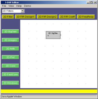
Fig. 1 2D J-DSP.
Let’s start with a
simple two-dimensional (2-D) J-DSP simulation.
Exercise 1.1
First, place the 2D SigGen
block in the workspace of the J-DSP editor as shown in Fig. 1. Double click on
the 2D
SigGen block to open the
main dialog box. In this dialog box, you will find a list of different
pre-defined signals with editable horizontal and vertical widths as shown in
the Fig. 2. The user can perform some basic operations on the defined/selected
signal by going into the Customize
dialog box, and one can also edit/view the numerical values of the signal by
clicking on the [Edit Signal] in the Customize
dialog box.
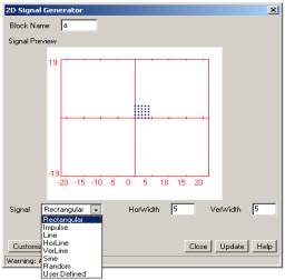
Fig.2 Main dialog box for 2D SigGen.
Exercise 1.1.1
Once you have opened the main dialog box of the 2D SigGen block, set
- Signal
Type = “Rectangular”
- Horizontal
Width = 5
- Vertical Width = 4
Click
on [Update].
Your
signal will look as shown in Fig. 3.
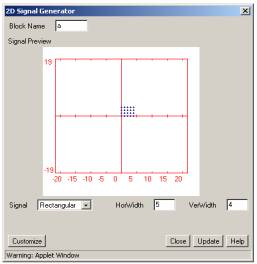
Fig.3 Main dialog box for 2D SigGen after [Update].
Note:
Clicking on the [Update] button is very essential, not only for the changes to
take effect but later you will see it is also required for the new data to be
transferred to the next attached block.
Now click on the [Customize] button in the main dialog box. A new dialog box will open as shown in Fig. 4(b).
Change the values in the shift fields as follows:
- Shift in
n1 direction = -3
- Shift in
n2 direction = 2
Click
on [Update].
The
position of blue dots in the main dialog and some values in the Customize dialog box will change and are
shown in Figs. 4(a) and 4(b) respectively.
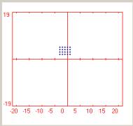
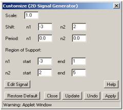
Fig.
4(a) “Rectangular” signal after shift. Fig. 4(b) Customize dialog after shift.
Look at the values in the “Region of support” (ROS)
fields. These values changed because ROS is usually taken to be the smallest
rectangular region that contains all non-zero values/samples in the
signal/sequence.
Before going to the next step, adjust all the dialog boxes,
which you have opened so far, in such a way so that you can see all of them at
the same time.
Exercise 1.1.2
Now click on the [Edit Signal] button in the Customize dialog. This will open the Edit dialog box that shows the numerical
values of the data samples in the region of support shown as blue dots in the
main dialog box.
Let’s try to insert a point at:
- (n1, n2) = (2, 2)
- Value = 1
But
this time click on [Apply], instead of [Update].
The
Edit dialog box will look as shown in
Fig. 5.
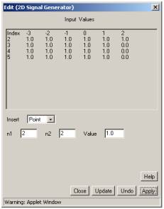
Fig. 5 Edit dialog
box after inserting a point at (2, 2).
Note
that the signal type in the main dialog has changed from “Rectangular” to
“User-defined” and compare the new values in the ROS fields with those shown in
Fig. 4(b).
Click
on [Undo] in the Edit dialog box to
go back to the previous settings. You will find your “Rectangular” signal back.
Close the Edit dialog.
Exercise 1.1.3
In the Customize
dialog, set
- Period in
n1 = 10
- Period in
n2 = 8
Click
on [Update].
Look
at the numerical values in the Edit dialog that shows the values in one
period of the periodic signal. Close this dialog box.
Exercise 1.1.4
Set the parameters in the Customize dialog box as,
- Period in
n1 = 4
- Period in
n2 = 8
Click
on [Update].
Again,
open the Edit dialog box to see the
values.
a)
What change did you
observe in the signal values?
b)
Does this remind you
of aliasing/overlapping? Give reason.
c)
What are the
precautions one should take to avoid aliasing?
Click on [Restore Default] in the Customize dialog, you will find your original “Rectangular” signal
back.i.e., all the values are set to their initial default ones for that
particular signal. Before going to the next part, close all the dialog boxes.
Connecting different blocks
Exercise 1.2
Until
now, we have been working on a single block. Let’s connect some of the blocks
together. There is a 2D Plot block in the
permanent blocks. Click on it and drag it in the workspace of the J-DSP editor.
Your workspace now contains two blocks as shown in Fig. 6(a).
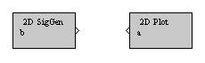
Fig. 6(a) J-DSP editor workspace after placing 2D plot block.
Exercise 1.2.1
As
you can see, 2D SigGen
block has one outlet/output-node and 2D Plot has one inlet/input-node. If you click on the output node
of the 2D
SigGen block and drag it to
the input node of the 2D Plot, it will
establish a connection between the two blocks as shown in Fig. 6(b). Now what
has happened internally? The 2-D signal that you have generated in the 2D SigGen block will transfer to the 2D Plot block. Double-click on the 2D Plot block and set:
- Mode of
display = “Samples”
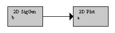
Fig. 6(b) J-DSP editor workspace after making connection
between the two blocks.
If you don’t see any
signal, you need to re-open the 2D SigGen
block and press [Update] button in the main dialog box.
Note: Whenever you
make/establish a connection between any two blocks, you need to press [Update]
button in order to transfer the signal/data to the next block.
If you click on the [Values] button
in the 2D
Plot dialog box, another
dialog window pops up that shows the values transferred from the 2D SigGen block to the 2D Plot. Fig. 7 shows
the dialog window in the 2D Plot block, when
“Line” was selected in the 2D SigGen
block.
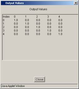
Fig. 7 Dialog window in the 2D plot block.
Now
if you make your signal periodic, the 2D Plot block will show the same periodic signal in the main dialog
box of the 2D Plot block, but
the Values dialog will show only the
values in one period.
Exercise 1.3
Let’s try to work on a very basic 2-D arithmetic operation.
First, click on the connection between the 2D SigGen and 2D Plot blocks and
hit the “Delete” button on your keyboard. Place 2D Arith and another 2D SigGen
block as shown in the Fig. 8(a).
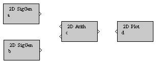
Fig. 8(a) J-DSP editor workspace after placing 2D Arith and another 2D SigGen
blocks.
Exercise 1.3.1
Establish the connections between the blocks in the similar
fashion as you did in the exercise 1.2.1. Your current J-DSP workspace should
look as shown in the Fig. 8(b).
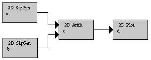
Fig. 8(b) J-DSP editor workspace after establishing
connections between the blocks in Fig. 8(a).
Exercise 1.3.2
Set the following signal settings in one of the 2D SigGen block.
- Signal
Type = “Line”
- Horizontal
Width = 6
- Vertical Width = 6
Click
on [Update].
Similarly,
in the second 2D SigGen
block set the following.
- Signal
Type = “Rectangular”
- Horizontal
Width = 3
- Vertical Width = 3
Click
on [Update].
Double
click on the 2D Arith block and
select,
- Arithmetic
Type = Addition
Click
on [Update].
To
see the final values, double click on the 2D Plot and click on the [Values] button in it.
a)
Does this arithmetic
operation change the ROS of the input signals? If yes, how?
Exercise 1.3.3
Now work on the same system as in fig. 8(b) and use the same
“Line” signal as in the last step, but make the following changes in the above
“Rectangular” signal.
- Shift in
n1 direction = 2
- Shift in
n2 direction = 2
Click
on [Update].
Double
click on the 2D Arith block and
select,
- Arithmetic
Type = Multiplication
Click
on [Update].
a)
What is the ROS of
the output signal? How it is calculated?
This
concludes the introduction to 2-D J-DSP.