On-line
Computer Laboratories with J-DSP
by
Andreas
Spanias
Preliminary Sample
Lab 1: Working with J-DSP
Please Perform and Provide Evaluation
at
http://jdsp.asu.edu/evaluation
General Information on J-DSP
All functions
in J-DSP appear as graphical blocks that are divided into groups according to
their functionality. Selecting and establishing individual blocks is done using
a drag-and-drop-process. Each block
is linked to a signal processing function. Figure 1 shows the J-DSP editor
environment and Fig. 2 shows details on the drop-down menus and the signal
processing functions of J-DSP. A simulation can be started by connecting
appropriate blocks from left to right. Signals at any point of a simulation can
be analyzed and plotted through the use of appropriate functions. Parameters in
the blocks can be edited through dialog windows. Blocks can easily be manipulated (edit, move,
delete and connect) using the mouse. Execution is dynamic and therefore any
change at any point of a simulated system will automatically take effect in all
related blocks. Select windows can be left open to enable viewing results at
more than one point in the editor.
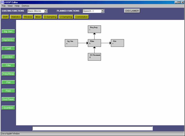
Fig. 1. The J-DSP
simulation environment
Lab 1: Working with J-DSP
The
easiest way to explain some of the functions of J-DSP is to work through a
simple example. To start J-DSP, go to
the link http://jdsp.asu.edu/, click on “Start
J-DSP”, and press “start" in the subsequent dialog window. When the start
button is pressed and you attempt to establish your first block a relatively
large Java applet will start downloading to the browser. Therefore it may take
30 seconds or more to establish the first block for a telephone-based (28.8)
internet connection but once the first block is established the program should
run reasonably fast. Adjust the size of the J-DSP editor window so that
you are able to view the entire work area. Press the SigGen button on the left
part of the window. Move the mouse to the center of the window and click
the left mouse button. Note that you have created the signal generator
block. There are two signal generators, SigGen for processing a
single frame of the signal and SigGen(L) for frame-by-frame processing
that is typically used in speech processing simulations. Similarly, create a Filter
and a Plot block, Fig. 3. Note
that blocks cannot be placed on top of one another. There are two plot blocks,
i.e., Plot (single plot) and Plot2 (two plots). For now, use Plot.
Fig. 3. J-DSP buttons for a source-filter
simulation.
Note that each block has signal input(s), designated by the small triangular nodes, on the left and signal output(s) to the right. Some blocks carry parameter inputs and outputs at the bottom and top of the block respectively. For example, the Filter block has a coefficient input on the bottom and a coefficient output on the top. To select a block, click once to highlight it. You can then move it by placing the mouse arrow over it, holding down the left mouse button and dragging the box to a new location. To delete a block, simply select it and press the "delete" key on your keyboard. To link blocks, click once inside the small triangle on the right side of the signal generator box and while holding the mouse button down, drag the mouse arrow to the triangle on the left side of the filter box. Release the mouse button to create a connection between the two boxes. Always make the connections in the direction of the signal flow. The Coeff. block is used to specify filter coefficients. The block is connected to the Filter block parameter input as shown below. Now, connect the Filter block to the Plot block so that your editor window looks like the block diagram. Note that you can view the dialog box of each block by double-clicking on the block, as shown in Fig. 4.
Fig. 4. Dialog windows in J-DSP.
|
Fig. 4. Dialog windows in J-DSP. |
Choosing Signals
Let us
now form a signal using the signal generator. Double click inside the Sig
Gen box and a dialog window
will appear, Fig. 5. If you do not see a
dialog window, you are using an older Internet browser and must download the newest
version of Netscape or Internet Explorer and start over. Use Internet Explorer
5.5 or later, or Navigator version 4.6 or later, with its Java plug in.
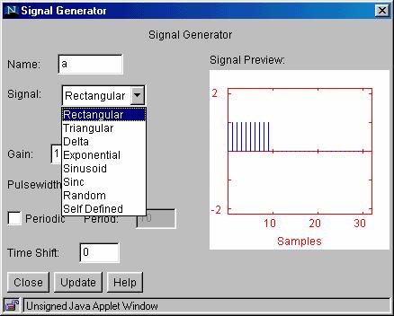
Fig. 5.
Signal generator dialog
On the
right side of the signal generator window, you can see a preview of the signal.
You may change the “name” of the signal, the “gain”, the “pulse width”, the
“period” and the “time shift” by typing the desired value into the appropriate
box. The signal type can be changed by
clicking on the pop down menu and selecting a signal. If you select a User-defined signal, an [Edit
signal] button will appear allowing you to edit the signal. With all signals except audio, J-DSP assumes
a normalized sampling frequency of 1Hz.
Hence the sampling frequency in terms of radians is 2p. All frequencies are entered as a function of p,
e.g., 0.1p, 0.356p, etc. Any sinusoidal frequency at or above p
will result in aliasing.
Step 1.1:
Create
a sinusoid with “frequency” 0.1p, “amplitude” 3.75, “pulse
width” 40. When all of the parameters
have been entered, press the [update] button to update the signal preview.
Remember that whenever changes are made to this box, the [update] button must
be pressed in order for the changes to take effect. On the right, you can see a
preview of the input signal. Count the number of samples within a period. How
many do you have? (ans: 20 samples).
Step 1.2: Create a sinusoid with “frequency” p,
“amplitude” 3.75, “pulse width” 40 (remember to press update for changes to
take place). What happens? (ans: we have
aliasing, i.e, no signal).
Step 1.3: Create a sinusoid with “frequency” 1.3p,
“amplitude” 3.75, “pulse width” 40. What
happens? Count the number of samples in
a period. (ans: we have aliasing again , signal makes no sense).
Step 2: Next,
we want to take a look at the Filter output in the time and
frequency domain. Set the values in Sig
Gen as per step 1.1.
Double-click the Plot block and a new dialog window
will appear. You should again see the
input signal because the filter is just letting the signal pass through
unaffected, since no coefficients have been set. If you press the [Graphs/Values/Stats]
button, a table with the values of the signal pops up. In the first column you see the indices of
the samples and the second column shows you the values. Close the value dialog box.
Step 2.1 Let us now see the filter in action. Keep the Plot window open to observe any
changes. Double click the Coeff.
block. You should see the following (Fig. 6):
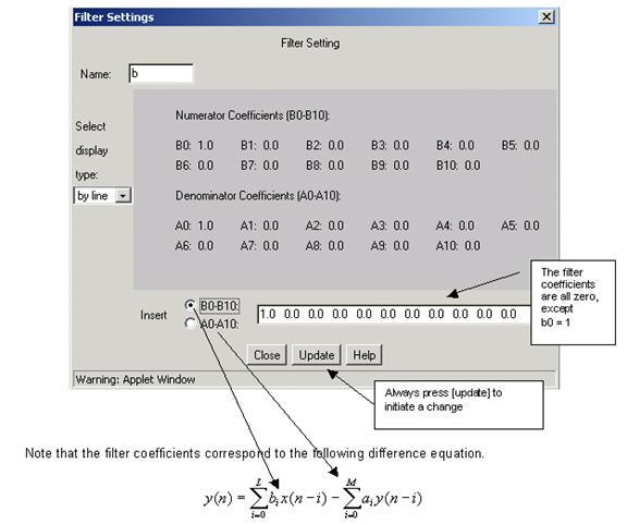
Fig. 6.
Coefficient entry in J-DSP
Step 2.2 Keep the values in Sig Gen as per step 1.1.
Change the filter coefficient to b0=4 and press [update]. Double
click on the Plot block. You should see that the amplitude of the sinusoid
has changed (ans: peak amplitude 4x3.75= 15).
Step 2.3: Implement a pure delay by setting b5=1
and rest of the coefficients (including b0) to zero and press [update]. What
happens to the sinusoid?
Step 2.4 Implement a simple LPF, set b0 =
0.2 and a1 = -0.8 and press [update]. Generate a sinusoid with “gain” 1,
“frequency” 0.1p, “pulse width” 256. What do you observe?
What
kind of signal do you get at the output? Why? What is the peak-to-peak value?
Do we have a change? Is there a phase shift? What filter function determines
the time shift?
Step 2.5: Select the Freq-Resp block from the
panel of general blocks on the left of the window and place it to the north of
the Filter
block. Connect the parameter output to the Freq-Resp block. Double click the Freq-Resp
block. You should see the magnitude and phase response of the filter. Change
the coefficient to a1 = 0.8 instead of a1 = -0.8. What do
you see in the frequency response and output?
(ans: HPF, decrease in amplitude)
Step 3: To view the signal in the frequency domain, insert an FFT box between the Filter and the Plot box as shown below. The FFT box can be found under the Freq. Blocks menu.
Fig. 7.
Source-filter simulation with FFT at the output
Step 3.1 Set the Filter parameters and input as per
step 2.4. Double click on the FFT
block and change the “FFT size” to 256 points and then press [Close]. Now, you can see the magnitude and the phase
of the signal in the frequency domain.
The magnitude has a sharp peak approximately at 0.31, the frequency of
our sinusoidal signal (0.1x3.1459).
Step 3.2 Change the sinusoidal frequencies as per
steps 1.2 and 1.3 but with “pulse width” 256. What do you observe?
Step 3.3 Delete the filter. Set the sinusoidal “frequency” in Sig Gen as per step 1.1 but with “pulse width” 256. Now create a second Sig Gen block and a Mixer block. Your editor window should then look like the following:
Fig. 8.
Sinewave plus noise simulation
Change
the name of the first Sig Gen block to ‘Sinusoi’, the
second Sig Gen block to ‘noise’ and the Plot block to
‘SigNoi’. The names are restricted to
six characters. Following that, we edit the Sig Gen block called
‘noise’. Open the dialog window and
change the “signal type” to “random”. Choose a “variance” of 4 and extend the
“pulse width” to 256 samples, in order to have noise over the full length of
the signal. Now take a look at the output
signal. In the time domain it is very
hard to see that a sinusoid is present.
However, if you view the signal in the frequency domain with an FFT size
of 256, then you still find a peak at approximately 0.31.
Step 3.4: Change the amplitude of the sinusoid up or down and observe the spectra (FFT plot). Try different values to make the sinusoid to dominate the noise signal or be masked by the noise signal. Remember the movie “The Hunt for Red October" which was about a stealth Soviet sub-marine defecting? In that movie they showed sonar operators viewing FFT spectra and listening to sonar signals as they were searching for submarine propeller signatures (quasi-periodic signals) in ocean noise (random broadband signals). Stealth submarines have, among other things, weak broadband propeller signatures that can be masked easily by ocean noise.